Peeking Inside Diffusion Language Models with LogitLens

Lately, diffusion-based language models like LLaDA and MMaDA have been gaining traction. These aren’t your standard left-to-right text generators - they’re bidirectional models trained to fill in missing tokens, more akin to BERT but on steroids. During training, Diffusion Language Models (DLMs) learn to predict <mask> tokens given context, effectively learning a denoising task.

In this post, we’ll explore how DLMs work “under the hood” using one of the most elegant interpretability tools out there: LogitLens. The final result will be a plot like this one, that we obtained applying LogitLens to Llama in a previous blog post.

As usual, here is the code to reproduce all the plots, just

A Quick Refresher: What Is LogitLens?

LogitLens is a clever interpretability method originally designed for autoregressive (AR) LLMs. Instead of applying the final language modeling head only to the last hidden layer (as is standard), LogitLens applies it at every intermediate layer. This lets us “see” how predictions evolve across layers—like watching a thought form in real time.

In a previous blog, I showed how to implement LogitLens for LLMs from scratch. This time, we’ll use it to analyze DLMs—specifically LLaDA and Dream—to observe how they construct predictions layer by layer. I should mention here that this is not the most advanced interpretability method (e.g. see this nice blog) but it still gives us cool insights into the model’s inner workings!

---

Setup: Probing LLaDA with a Simple Prompt

Let’s start by loading the LLaDA-8B model and giving it a classic prompt:

import torch
from transformers import AutoTokenizer, AutoModel

device = 'cuda'
model_name = 'GSAI-ML/LLaDA-8B-Base'
model = AutoModel.from_pretrained(model_name, trust_remote_code=True, torch_dtype=torch.bfloat16).to(device).eval()
tokenizer = AutoTokenizer.from_pretrained(model_name, trust_remote_code=True)

Now we create a simple prompt:

example = "The quick brown fox jumps"
prompt = tokenizer(example, return_tensors="pt").to(device).input_ids

Unlike GPT-style models that generate one token at a time, diffusion models generate N tokens simultaneously, where N is the number of masked tokens in the input sequence. This means they need to know the amount of masked tokens, that is, their target length, before they begin. We can think of it like filling out a crossword puzzle—you need to know exactly how many squares you’re working with before you can start placing letters. This might sound like a design problem for open ended generation (it kind of is) but we can circumvent with various strategies.

To prepare our input, we create a sequence with the original prompt + 8 mask tokens <mask>. The <mask> tokens are the squares of the puzzle the model has to fill in.

mask_id=126336 # specific to llada model
gen_length=8
x = torch.full((1, prompt.shape[1] + gen_length), mask_id, dtype=torch.long).to(model.device)
x[:, :prompt.shape[1]] = prompt.clone()

Just to make sure we see what we are doing, let’s visualize what is happening and print the input before feeding it to the model:

tokenizer.convert_ids_to_tokens(x[0], skip_special_tokens=False)

['The', 'quick', 'brown', 'fox', 'jumps', '<|mdmmask|>', '<|mdmmask|>', '<|mdmmask|>', '<|mdmmask|>', '<|mdmmask|>', '<|mdmmask|>', '<|mdmmask|>', '<|mdmmask|>']

It makes sense, we have our prompt + the mask tokens the model will try to fill in.

Running the Model

Let’s forward the input through the model and grab the predicted tokens:

# we need all the intermediate hidden states
with torch.no_grad():
    outputs = model(x, output_hidden_states=True)

# get the predicted tokens and decode them
predicted_token_ids = outputs["logits"].argmax(-1)
tokenizer.convert_ids_to_tokens(predicted_token_ids[0], skip_special_tokens=False)

['_', 'quick', 'brown', 'fox', 'jumps', 'over', 'the', 'lazy', 'dog', '.', '_', '_', 'jumps']

Well, after just one decoding step we were not expecting any special results. Usually, we perform at least N/2 denoising steps, where N is the generated sequence length. However, we see the model has already guessed (correclty) almost all the missing words. On the other hand, the first token The has been replaced by a _, which we don’t mind as being part of the prompt we would just ignore that during decoding. If you want to get a better prediction, you should perform additional diffusion steps, by remasking some of the input tokens. This is out of the scope for this blog, as we just want to explore the inner representations of the model.

Logit Lens

We just got the predictions fot the final output of the model, that is, what comes out of the last layer. What if we apply the model head (our “Lens”) to intermediate representations though? Intermediate representations are stored in the outputs.hidden_states. We’ll have one for each layer of the model and each token of the sequence.

logitlens = []

for hidden_state in hidden_states:
    hidden_state = model.model.transformer.ln_f(hidden_state)
    logits = model.model.transformer.ff_out(hidden_state)
    # get predictions for this layer
    predicted_token_ids = logits.argmax(-1)
    predicted_tokens = tokenizer.convert_ids_to_tokens(predicted_token_ids[0], skip_special_tokens=False)
    # store in our logitlens list
    logitlens.append(predicted_tokens)

Now the list contains decoded sequences for each layer. For instance, if we want to check what the model was “thinking” at layer 5, we can just do:

print(logitlens[5])

['paralleled', 'awaited', 'funnels', 'gfx', 'tesy', 'awaited', 'awaited', 'blockList', 'blockList', 'blockList', 'blockList', 'blockList', 'blockList']

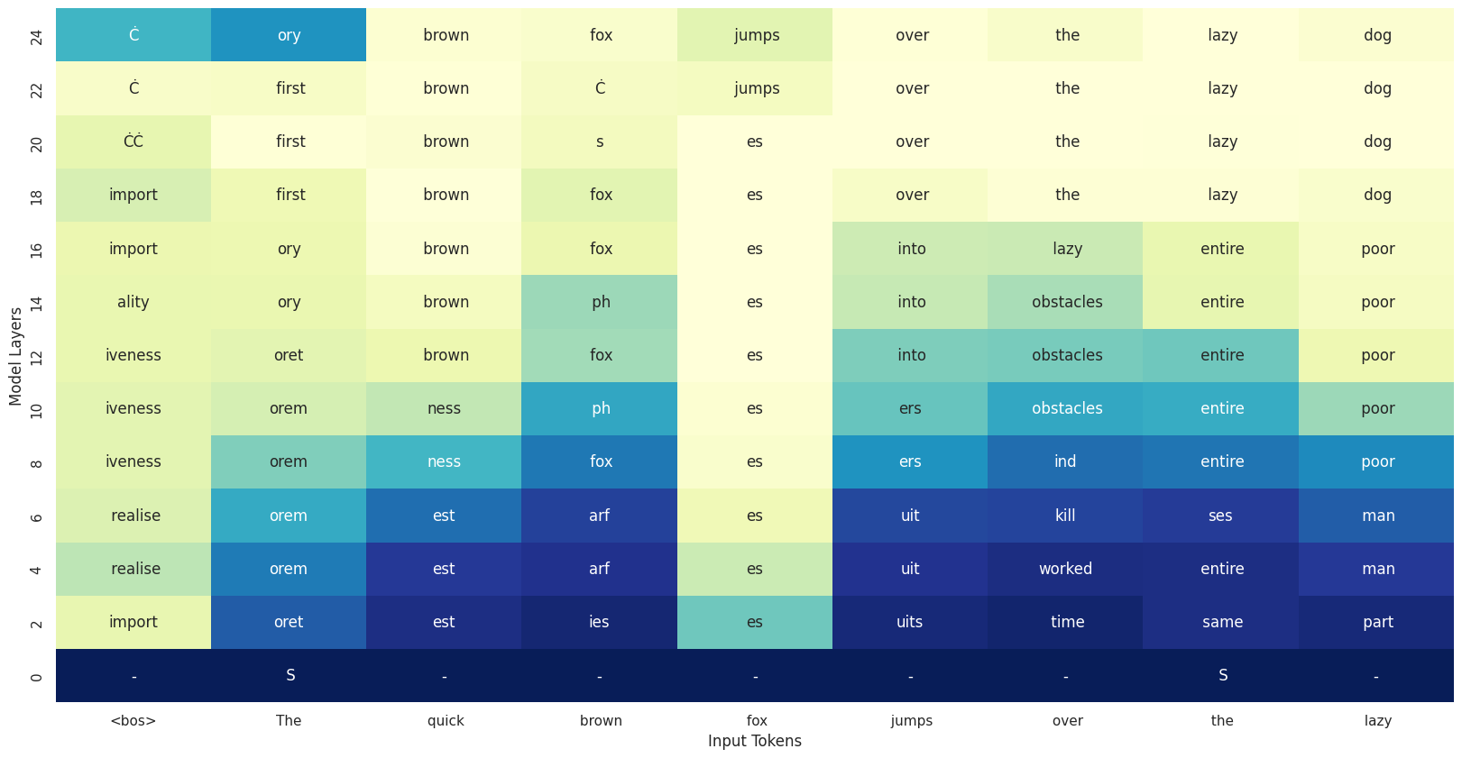
The raw output appears chaotic and difficult to interpret. To better understand the model’s internal reasoning process, let’s visualize the complete sequence predictions across all transformer layers using a heatmap (full implementation available in the accompanying notebook).

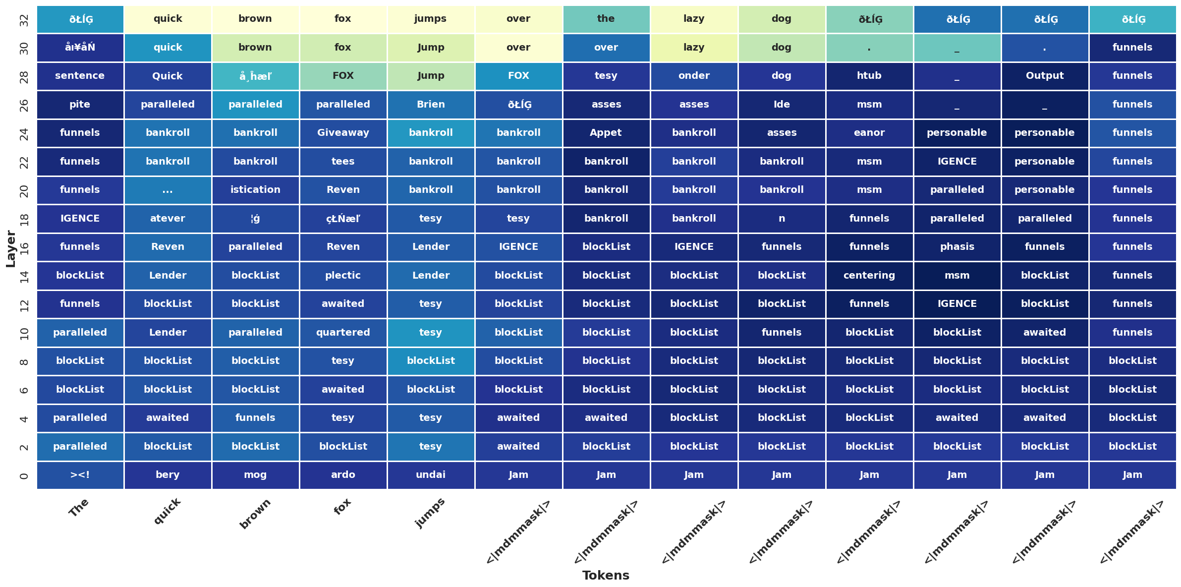
The bottom row shows the original input tokens, while each ascending row represents successive transformer layers from early to final. The color intensity indicates entropy ( ~ prediction confidence) at each layer, with darker cells representing higher entropy (model uncertainty) and brighter cells showing lower entropy (confident predictions). – that is why brighter cells are only in the final layers.

A few thoughts

The most evident pattern is that coherent, confident predictions only emerge in the final layers, typically around layer 25 and beyond. Throughout the majority of the network depth, the model remains highly uncertain about its predictions, as evidenced by the prevalence of darker cells (and wrong tokens) in earlier layers. Additionally, correct tokens only emerge at the very final layer. This behavior fundamentally differs from autoregressive models like LLaMA or Gemma, where confident predictions typically crystallize much earlier in the network.

This behavior might be caused by a lot of factors. Keeping in mind that logit lens can be deceiving as it depends intermediate layer’s basis vector alignment with the output space, we can conjecture that the model is performing a lot of computation that is not interpretable in intermediate layers, and creating semantic representation only in the final ones. This might be a consequence of the bidirectional attention (implies more “mixing” of the tokens hence more overlapped signals?).

Alos, we should not forget taht we’re observing only the first denoising step of what is inherently a multi-step iterative process. The model is designed to gradually refine predictions across multiple iterations, so initial uncertainty and errors are not only expected but necessary for the denoising mechanism to function properly. More precisely, the more mask tokens, the harder the task hence the uncertainty for the model.

Testing on Dream

Finally, let’s repeat the process with Dream (check the Colab for the full code). Here, I will plot fewer layers to make them more clear:

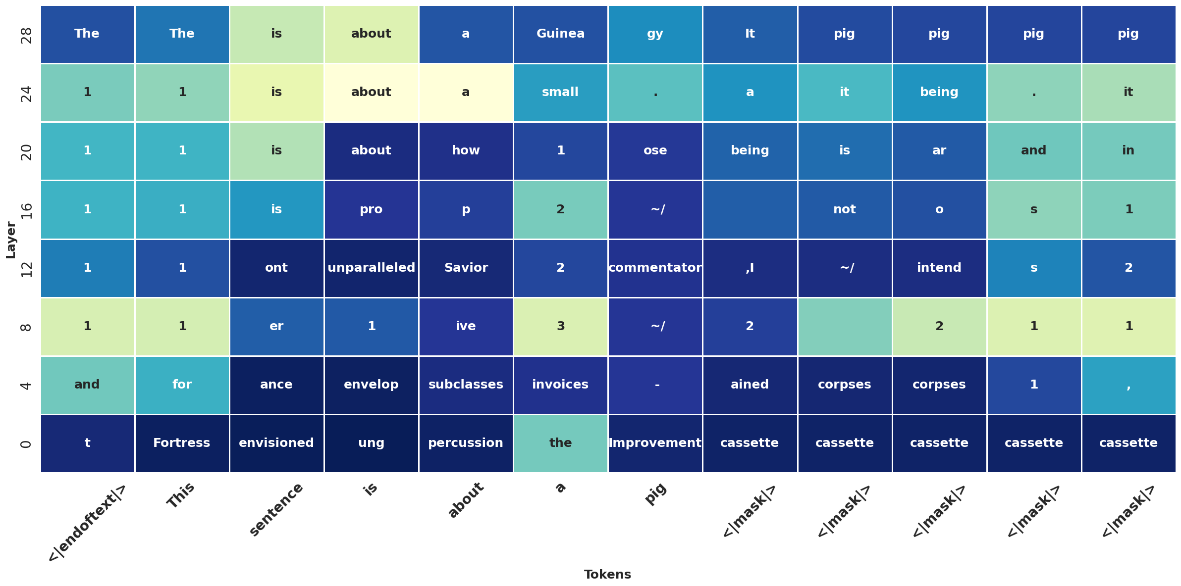
It looks like Dream gets more confident at early layers, but still, correct predictions only emerge very late. In this plot, it’s also worth to point out an interesting behavior that we didn’t observe in the previous example: DLMs ability to “peek into the future”. If we look carefully, Dream predicts tokens related to words that come later in the sequence, which would be impossible in autoregressive models, where each token only attends to previous ones. An example is the token “Guinea” emerging before “pig” (I’m assuming the sentence “this sentence is about a Guinea pig” is not present in the training corpus here). With bi-directional attention, all tokens attend to each other from the start, enabling DLMs to make globally-informed guesses during decoding!

That’s it! If you have feedback, want to chat about this topic, or find bugs in the code, feel free to reach out on Twitter or any social platform. Thanks for reading!