
Efficiency Metrics in Machine Learning
In the world of machine learning, efficiency is a buzzword we hear all the time. New methods or models often come with the claim of being more efficient than their predecessors. But what does “more efficient” actually mean? Comparing efficiency objectively can be tricky since the metrics used to measure it are often confusing and varied. Some are hardware-dependent, while others are not. Some concern the memory and the compute, while others the power consumption.
For instance, latency and throughput are critical for evaluating how well a model performs in real-time applications during inference. On the other hand, floating-point operations per second (FLOPs) and parameter size are often considered during the training phase to gauge the computational and memory demands of a model.
In this short post, I will recap the most important metrics used to measure efficiency of models and highlight their differences.
Parameters size
The number of parameters in a model refers to the total count of learnable weights. A higher number of parameters can lead to a more powerful model capable of capturing complex patterns. However, it also demands more memory, which can make training and deployment challenging. In the past recent years, large language models (LLMs) have become extremely popular. LLMs can contain huge number of parameters, often running into billions.
Here we provide a simple table containing the number of parameters in most popular neural network layers, assuming we have an input with \(c_i\) channels, and an output with \(c_o\) channels. For convolutions, we denote the height and width of the kernel with \(k_h, k_w\) respectively.
| Layer | Number of Parameters (bias is ignored) | Explanation |
|---|---|---|
| Linear Layer | \(c_o \cdot c_i\) | simply the number of edges in a fully connected |
| Convolution | \(c_o \cdot c_i \cdot k_h \cdot k_w\) | for each input channel we have a kernel \(k_h \times k_w \times c_o\) |
| Grouped Convolution | \(\frac{c_o}{g} \cdot \frac{c_i}{g} \cdot k_h \cdot k_w \cdot g = c_o \cdot c_i \cdot k_h \cdot k_w / g\) | we group convolutions into \(g\) groups |
| Attention Block | \(3 \cdot c_i \cdot c_o + c_o \cdot c_o\) | we first project into \(QKV\) and then perform output prjection |
It is important to point out that the number of parameters does not coincide with the actual memory required to store the model, as this depends on the floating point precision. Floating point precision determines how many bits we use to store each parameter. As a consequence, the final size of the model can be computed as:
\[\text{Parameters size} = \text{number of parameters} \times \text{parameter size}\]We often try to use as few bits as possible to represent model weights, which is called quantization. Quantization reduces the precision of the model’s parameters, typically from 32-bit floating-point to 16-bit or even 8-bit integers, significantly decreasing the memory footprint and computational requirements.
As an example, the size of llama3-8b in standard fp16 would be roughly \(8000000000 \times 16 bits \sim 16 \text{GB}\). If we employ int4 quantization, the size goes down to \(8000000000 \times 4 bits \sim 4 \text{GB}\) !
The parameters size is independent from the underlying hardware, and impacts the memory during training (we have parameter efficient fine-tuning methods to tackle that) and inference (quantization helps a lot here). Additionally, as a general rule, a model with fewer parameters generally requires less compute, so parameters size often indirectly affects computational demands.
MACs and FLOPs
MACs (Multiply Add operations) and FLOPs (Floating Point Operations) measure the computational effort required to execute a function. One MAC is defined as:
\[a = a \times b + c\]One MAC requires performing one multiplication and one addition, i.e. two generic Floating Point Operations. Hence, we have that \(FLOPs = 2 \times MACs\).
MACs and FLOPs provide a hardware-independent way to estimate the computational cost, allowing comparisons across different models and architectures. Lowering the FLOPs while maintaining model performance is a common goal, as it can lead to faster inference times and lower energy consumption, making the model more suitable for deployment in resource-constrained environments.
However, it’s important to note that lower FLOPs do not necessarily translate to lower latency. For example, a model might have fewer FLOPs but require more memory access operations, which can be slower than the arithmetic computations themselves. Conversely, a model with higher FLOPs might be highly optimized for parallel processing, leading to lower latency on specific hardware. Thus, while FLOPs are a valuable metric for assessing computational cost, they should be considered alongside other metrics like latency to get a comprehensive view of a model’s efficiency.
In neural networks we perform a lot of matrix - matrix multiplications. For a matrix-matrix multiplication between \(A_{m \times n} \times B_{n \times k}\) we need \(nmk\) MACs and \(2nmk\) FLOPs. You can use this tool to count the FLOPs of a model in Pytorch. Let’s take a look at the FLOPs required by each of the most common neural networks layers.
| Layer | MACs | Explanation |
|---|---|---|
| Linear Layer | \(c_o \cdot c_i\) | vector matrix multiplication |
| Convolution | \(c_o \cdot o_w \cdot o_h \cdot c_i \cdot k_h \cdot k_w\) | for each output pixel, we perform the convolution \(k_h \times k_w \times c_i\) |
| Grouped Convolution | \(\frac{c_o}{g} \cdot o_w \cdot o_h \cdot c_i \cdot k_h \cdot k_w\) | we group convolutions into \(g\) groups |
| Attention Block | \(3 \cdot N \cdot {c_i}^2 + N^2 \dot c_i + N^2 \cdot {c_i}^2\) | QKV projection + attention computation + output projection |
FLOPs determine the computational intensity of model, and are the factor that most prominently affects the compute resources. The number of FLOPs that a the specific hardware can perform in a second, i.e. FLOPs per Second, is called FLOPS and measures hardware performance.
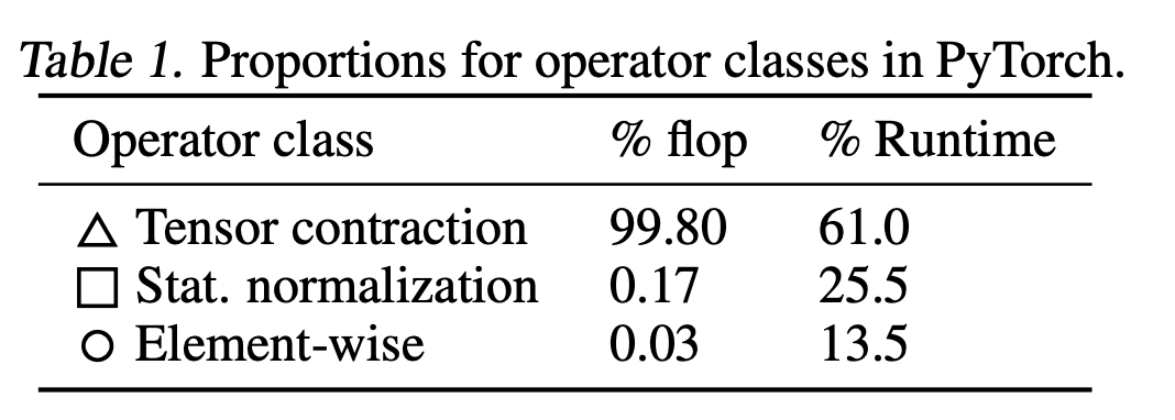
A side note on matrix multiplication. Modern GPUs are super-optimized for matrix multiplication, while other operations (e.g. layer normaliazions et similia) are less optimized. Still, this is not a problem as modern deep learnign models rely a lot on matrix multiplications. As a case study, this is how the FLOPs for a Bert model are distributed among classes of operations (credit):
Latency
Latency refers to the time it takes for a model to process an input and produce an output. This metric is particularly important in real-time applications, where quick responses are critical. High latency can lead to poor user experiences or even system failures in safety-critical applications.
Latency is highly dependent on three factors: the number of parameters in the model, the FLOPs required by the model, and hardware specific constraints. Because latency is extremely hardware dependent, it is often not a good choice for comparisons. However, it is the most crucial metric for real world applications.
During inference and training, a typical machine learning data path involves: (1) reading data from memory to the streaming multiprocessors on the GPU core (2) performing the required computations and (3) writing the results back to memory, which can happen asynchronously thanks to the GPU’s VRAM supprting async I/O. Hence, we have two possible bottlenecks: the computation that takes place on the GPU cores (\(T_{compute}\)), or the memory input/output (\(T_{compute}\)). The latency of an operation is therefore determined by the “slowest” of these two steps.
\[\text{latency} = \max(T_{memory}, T_{compute})\]If \(T_{memory} > T_{compute}\) we say the operation is memory-bound, else we say it is compute-bound. How to find out \(T_{memory}\) and \(T_{compute}\) for a specific neural network layer? \(T_{compute}\) is simply the amount of time the cuda cores need to perform the computations required. Assuming our layer performs a given amount of FLOPs, and the GPU can perform at most Floating Point Operations per Second, we have that
\[T_{compute} = \frac{layer FLOPs}{GPU FLOPS}\]Notice that the maximum GPU FLOPs depend on the precision we are operating at, so FLOPs at fp16 are not the same as FLOPs at int8.
The \(T_{compute}\) is determined by the amount of data we have to move from memory, usually High Bandwidth Memory (HBM) and the memory bandwidth. When executing a layer, we need to read from memory (a) the layer parameters and (b) the input activations. Therefore, we have that
\(T_{memory} = \frac{\text{size of model parameters} + \text{size of input activations} + \text{size of output activations}}{\text{memory bandwidth}}\) Again, the size of parameters is determined by the precision at which we are operating.
Throughput
Throughput measures the number of inferences or predictions a model can make in a given time frame, usually one second. For an image classification task, these might be the number of images the model can classify in one second. While throughput is highly related to latency, they are not necessarily proportional. In order to increase throughput, we migh simply buy more GPUs and so get the chance to process more data in parallel, while the latency for a single input-output stays the same.
Energy Consumption
Energy consumption measures the energy required to perform an operation. This metric has gained increasing importance due to the environmental impact of large-scale machine learning and the operational costs associated with running models. Energy-efficient models not only reduce the carbon footprint but also lower the operational expenses for businesses deploying machine learning solutions. Techniques to minimize energy consumption include optimizing algorithms, utilizing energy-efficient hardware, and adopting more sustainable practices in data centers. Recent work has proposed models to estimate the carbon footprint for training models.
Additionally, energy is crucial for on-device training, which is necessary for all those scenarios where data cannot be shared due to privacy concerns. Unlike inference, training requires significant computational resources to adjust the model’s parameters. However, the computational and energy resources offered by edge devices are often scarce.
In general, VRAM memory access is the most energy consuming operation, requiring 100x more power than accessing SRAM and 200x than performing an ADD operation.
Peak Activations
Peak activations refer to the maximum memory occupied by activations (outputs) produced by neurons in the network during the forward propagation process. At inference time they do not represent a significant bottleneck, because (a) the batch size it typically small and (b) we don’t need to store them for backpropagation. During training, the activations represent the most significant bottleneck, because we need to store them for gradient computation to update model weights.
It is important to point out that only activations of nonlinear layers introduce this problem. Assuming we have a layer \(a_{i+1} = \mathbf{w_i}^T a_i + b\). At some point during backprop, we need to compute the gradient of loss with respect to the activations \(a_i\). Applying the chain rule, we have that:
\[\frac{\partial \mathcal{L}}{\partial a_i} = \frac{\partial \mathcal{L}}{\partial a_{i+1}} \frac{\partial a_{i+1}}{\partial a_i} = \frac{\partial \mathcal{L}}{\partial a_{i+1}} \mathbf{w_i}^T\]if the layer is linear, whereas we have
\[\frac{\partial \mathcal{L}}{\partial a_i} = \frac{\partial \mathcal{L}}{\partial a_{i+1}} \frac{\partial a_{i+1}}{\partial a_i} = \frac{\partial \mathcal{L}}{\partial a_{i+1}} \mathbf{g}(a_i)\]where \(\mathbf{g}(a_i)\) depends on the activations at previous layer. This means that for a nonlinear layer, we need to store all the activations.
Model FLOPs utilization
Model FLOPs utilization was proposed by Google as a metric to capture how well a specific model is using the hardware available. More specifically, it is defined as the ratio between the observed output throughput and the maximum theoretical throughtput.
\[\text{MFU} = \frac{Achieved FLOPs/s}{Theoretical Peak FLOPs/s}\]Importantly, the maximum theoretical throughput only accounts for FLOPs (forward and backward) and not for rematerialization + other computational overhead. A low MFU means that the model is underutilizing the hardware due to inefficiencies such as memory bottlenecks, poor parallelism, or excessive communication overhead.
This is an extremely important metric saying a lot about our implementation and training pipeline, as it captures the number of FLOPs a model theoretically utilizes compared to hardware peak FLOPs.
| Metric | explanation | primarily affects | primarily affected by | hardware independent |
|---|---|---|---|---|
| Parameters size | memory footprint of model | latency, storage | model architecture & implementation, floating point precision | ✅ |
| FLOPs ( and MACs) | number of operations required by model | latency, energy | model architecture & implementation | ✅ |
| Latency | time required for one inference | end user experience | Parameters size, FLOPs, Hardware | ❌ |
| Energy | power consumed by operation | training/inference cost | model architecture, implementation | ❌ |
| Throughput | inferences per time frame | end user experience, energy | all | ❌ |
| Peak activations | memory occupied by outputs | training memory consumption | all | ✅ |